Kappa
“Great things are not done by impulse, but by a series of small things brought together.”
Hack The Box
Decision Trees
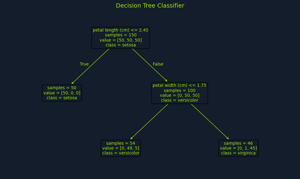
Decision trees are a popular supervised learning algorithm for classification and regression tasks. They are known for their intuitive tree-like structure, which makes them easy to understand and interpret. In essence, a decision tree creates a model that predicts the value of a target variable by learning simple decision rules inferred from the data features.
Imagine you're trying to decide whether to play tennis based on the weather. A decision tree would break down this decision into a series of simple questions: Is it sunny? Is it windy? Is it humid? Based on the answers to these questions, the tree would lead you to a final decision: play tennis or don't play tennis.
A decision tree comprises three main components:
- Root Node: - This represents the starting point of the tree and contains the entire dataset.
- Internal Nodes: - These nodes represent features or attributes of the data. Each internal node branches into two or more child nodes based on different decision rules.
- Leaf Nodes: - These are the terminal nodes of the tree, representing the final outcome or prediction.
Building a Decision Tree
Building a decision tree involves selecting the best feature to split the data at each node. This selection is based on measures like Gini impurity, entropy, or information gain, which quantify the homogeneity of the subsets resulting from the split. The goal is to create splits that result in increasingly pure subsets, where the data points within each subset belong predominantly to the same class.
Gini Impurity
Gini impurity measures the probability of misclassifying a randomly chosen element from a set. A lower Gini impurity indicates a more pure set. The formula for Gini impurity is:
          Gini(S) = 1 - Σ (pi)^2

          Where:
            S is the dataset.
            pi is the proportion of elements belonging to class i in the set.
Consider a dataset S with two classes: A and B. Suppose there are 30 instances of class A and 20 instances of class B in the dataset.
          Proportion of class A: pA = 30 / (30 + 20) = 0.6
          Proportion of class B: pB = 20 / (30 + 20) = 0.4
The Gini impurity for this dataset is:
Gini(S) = 1 - (0.6^2 + 0.4^2) = 1 - (0.36 + 0.16) = 1 - 0.52 = 0.48
Entropy
Entropy measures the disorder or uncertainty in a set. A lower entropy indicates a more homogenous set. The formula for entropy is:
          hbEntropy(S) = - Σ pi * log2(pi)

          Where:
            S is the dataset.
            pi is the proportion of elements belonging to class i in the set.
Using the same dataset S with 30 instances of class A and 20 instances of class B:
          Proportion of class A: pA = 0.6
          Proportion of class B: pB = 0.4
The entropy for this dataset is:
          Entropy(S) = - (0.6 * log2(0.6) + 0.4 * log2(0.4))
                     = - (0.6 * (-0.73697) + 0.4 * (-1.32193))
                     = - (-0.442182 - 0.528772)
                     = 0.970954
Information Gain
Information gain measures the reduction in entropy achieved by splitting a set based on a particular feature. The feature with the highest information gain is chosen for the split. The formula for information gain is:
          Information Gain(S, A) = Entropy(S) - Σ ((|Sv| / |S|) * Entropy(Sv))

          Where:
            S is the dataset.
            A is the feature used for splitting.
            Sv is the subset of S for which feature A has value v.
Consider a dataset S with 50 instances and two classes: A and B. Suppose we consider a feature F that can take on two values: 1 and 2. The distribution of the dataset is as follows:
          For F = 1: 30 instances, 20 class A, 10 class B
          For F = 2: 20 instances, 10 class A, 10 class B
First, calculate the entropy of the entire dataset S:
          Entropy(S) = - (30/50 * log2(30/50) + 20/50 * log2(20/50))
                     = - (0.6 * log2(0.6) + 0.4 * log2(0.4))
                     = - (0.6 * (-0.73697) + 0.4 * (-1.32193))
                     = 0.970954
Next, calculate the entropy for each subset Sv:
          For F = 1:
            Proportion of class A: pA = 20/30 = 0.6667
            Proportion of class B: pB = 10/30 = 0.3333
            Entropy(S1) = - (0.6667 * log2(0.6667) + 0.3333 * log2(0.3333)) = 0.9183
          For F = 2:
            Proportion of class A: pA = 10/20 = 0.5
            Proportion of class B: pB = 10/20 = 0.5
            Entropy(S2) = - (0.5 * log2(0.5) + 0.5 * log2(0.5)) = 1.0
Now, calculate the weighted average entropy of the subsets:
          Weighted Entropy = (|S1| / |S|) * Entropy(S1) + (|S2| / |S|) * Entropy(S2)
                           = (30/50) * 0.9183 + (20/50) * 1.0
                           = 0.55098 + 0.4
                           = 0.95098
Finally, calculate the information gain:
          Information Gain(S, F) = Entropy(S) - Weighted Entropy
                                 = 0.970954 - 0.95098
                                 = 0.019974
Building the Tree
The tree starts with the root node and selects the feature that best splits the data based on one of these criteria (Gini impurity, entropy, or information gain). This feature becomes the internal node, and branches are created for each possible value or range of values of that feature. The data is then divided into subsets based on these branches. This process continues recursively for each subset until a stopping criterion is met.
The tree stops growing when one of the following conditions is satisfied:
- Maximum Depth: - The tree reaches a specified maximum depth, preventing it from becoming overly complex and potentially overfitting the data.
- Minimum Number of Data Points: - The number of data points in a node falls below a specified threshold, ensuring that the splits are meaningful and not based on very small subsets.
- Pure Nodes: - All data points in a node belong to the same class, indicating that further splits would not improve the purity of the subsets.
Playing Tennis
Let's examine the "Playing Tennis" example more closely to illustrate how a decision tree works in practice.
Imagine you have a dataset of historical weather conditions and whether you played tennis on those days. For example:
PlayTennis  Outlook_Overcast  Outlook_Rainy  Outlook_Sunny  Temperature_Cool  Temperature_Hot  Temperature_Mild  Humidity_High  Humidity_Normal  Wind_Strong  Wind_Weak
----------  ----------------  -------------  -------------  ----------------  ---------------  ----------------  -------------  ---------------  -----------  ---------
No          False             True           False          True              False            False             False          True             False        True
Yes         False             False          True           False             True             False             False          True             False        True
No          False             True           False          True              False            False             True           False            True         False
No          False             True           False          False             True             False             True           False            False        True
Yes         False             False          True           False             False            True              False          True             False        True
Yes         False             False          True           False             True             False             False          True             False        True
No          False             True           False          False             True             False             True           False            True         False
Yes         True              False          False          True              False            False             True           False            False        True
No          False             True           False          False             True             False             False          True             True         False
No          False             True           False          False             True             False             True           False            True         False
The dataset includes the following features:
- Outlook: Sunny, Overcast, Rainy
- Temperature: Hot, Mild, Cool
- Humidity: High, Normal
- Wind: Weak, Strong
The target variable is Play Tennis: Yes or No.
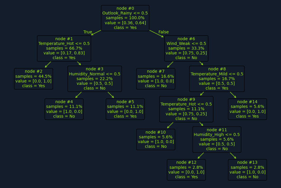
A decision tree algorithm would analyze this dataset to identify the features that best separate the "Yes" instances from the "No" instances. It would start by calculating each feature's information gain or Gini impurity to determine which provides the most informative split.
For instance, the algorithm might find that the Outlook feature provides the highest information gain. This means splitting the data based on whether sunny, overcast, or rainy leads to the most significant reduction in entropy or impurity.
The root node of the decision tree would then be the Outlook feature, with three branches: Sunny, Overcast, and Rainy. Based on these branches, the dataset would be divided into three subsets.
Next, the algorithm would analyze each subset to determine the best feature for the next split. For example, in the "Sunny" subset, Humidity might provide the highest information gain. This would lead to another internal node with High and Normal branches.
This process continues recursively until a stopping criterion is met, such as reaching a maximum depth or a minimum number of data points in a node. The final result is a tree-like structure with decision rules at each internal node and predictions (Play Tennis: Yes or No) at the leaf nodes.
Data Assumptions
One of the advantages of decision trees is that they have minimal assumptions about the data:
- No Linearity Assumption: - Decision trees can handle linear and non-linear relationships between features and the target variable. This makes them more flexible than algorithms like linear regression, which assume a linear relationship.
- No Normality Assumption: - The data does not need to be normally distributed. This contrasts some statistical methods that require normality for valid inferences.
- Handles Outliers: - Decision trees are relatively robust to outliers. Since they partition the data based on feature values rather than relying on distance-based calculations, outliers are less likely to have a significant impact on the tree structure.
These minimal assumptions contribute to decision trees' versatility, allowing them to be applied to a wide range of datasets and problems without extensive preprocessing or transformations.